Reference Functions in Excel

In my last post, I referred to some of the advanced Excel functions, the Excel post covered the N function, WILDCARDS, SUMPRODUCT, FREQUENCY, and ARRAYTOTEXT Functions. In this post, I will cover some reference functions that can help get the necessary information from the data and use the output for other functions to get the desired results.

What is Reference Function?

Reference functions are best used to get information from an array, indirectly represent the range from the dataset, and cross-reference different datasets. Most of the reference functions are defined within the hierarchy of the other functions as reference input.

Let's cover some of the reference functions that are used frequently for data analysis

• INDIRECT Function

The indirect function helps in manipulating the reference in a cell dynamically without changing the entire formula. The reference input is defined in a string format (in enclosed quotes).

Syntax:

INDIRECT (ref_text, [a1])

• ref_text - ​ref_text is defined in a string format, if not in an Error value the result will be #REF! Error value. Reference can contain A1- style or R1C1 style.

• [a1] optional - [a1] is used for representing A1-style or R1C1 style, by default or True represents A1 style of reference, and False represents the R1C1 style of reference.

Here are a few examples of the INDIRECT Function.

• ADDRESS Function

The Address function returns the address of a cell in the worksheet for the given row and column numbers, address function is used to represent the values in a cell indirectly or to find out the address of a value based on condition.

Syntax:

ADDRESS (row_num, column_num, [abs_num], [a1], [sheet_text])

• row_num - Numeric value that specifies the row number to use in the cell reference.

• column_num - Numeric value that specifies the column number to use in the cell reference.

• [abs_num] - Numeric value that specifies the type of reference to return.

Type of references for abs_num

1. or Omitted Absolute

2. Absolute row; relative column

3. Relative row; absolute column

4. Relative

• A1 Optional - Logical value that specifies A1 or R1C1 style, Null or True represents A1 style, and False R1C1 style reference.

• sheet_text - Optional String value to represent the name of the worksheet, only to be used as an external reference, the result of using the function will be "Sheet1! $A$1", if omitted the result will be an address of the cell in the current sheet.

Here are some examples of the ADDRESS Function.

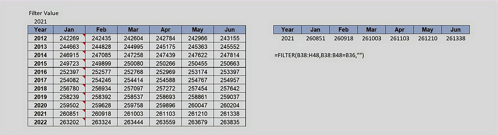
• FILTER Function

The filter function is the most used function for filtering the data. The filter function can be used to filter the data according to the criteria. This is most useful when trying to filter

Syntax:

 FILTER (array, include, [if_empty])

• Array - The array or range to filter.

• Include - A boolean array whose height or width is the same as the array.

• [if_emplty] - Value returning as a result of all values in the included array being empty.

Here are some examples of the FILTER Function.

• FORMULATEXT Function

This function returns the formula as a string, it is most useful when someone is looking to read the formula instead editing the formula using the F2 key. FORMULATEXT is useful if you are trying to explain any formula used in the sheet.

Syntax:

FORMULATEXT (reference)

• Reference - A reference to a cell or range of cells.

Here are some examples of the FORMUALTEXT Function.

• GETPIVOTDATA Function

This function returns the data from a Pivot Table, it is best used for gathering information from summarized data necessary for using as a source of input or displaying the result as an output.

Syntax:

GETPIVOTDATA (data_field, pivot_table, [field1, item1, field2, item2],...)

• data_field - Name of the PivotTable field that we need to retrieve, to be represented in quotes.

• pivot_table - Reference to any cell, range of cells, or named range of cells in a PivotTable.

• field1, item1 - 1 to 126 pairs of field names and item names that describe the data we want to retrieve.

Here are some examples of the GETPIVOTDATA Function.

• OFFSET Function

This function returns the range of cells or specified row and column number from a cell. The function helps extract the specified data in the range selected and can control the value seen at the output.

Syntax:

OFFSET (reference, rows, cols, [Height], [width])

• Reference - Reference refers to the range of cells or cells which we use as a base.

• Rows - The number of rows, Up or Down, UP can be represented by a negative of the numeric value, whereas Down can be represented by a Positive of a numeric value.

• Cols - The number of columns, Left or right, the Left can be represented by a negative of the numeric value, whereas the right can be represented by a positive of a numeric value.

• [Height] - The height in the number of rows, height must be a positive number.

• [Width] - The width in the number of columns, the width must be a positive number.

Here are some examples of the OFFSET function.

• ROWS Function

The rows function returns the number of rows in an array, rows function helps in counting the rows within the array, this function can be used as counting values in cells and is useful for the sequencing in a table, rows consider the first cell in a range as the first row.

Syntax:

ROWS (array)

• Array - An array or reference to a range of cells where we require a number of rows.

Here are some examples of the ROWS function.

• ROW Function

This function returns the row number of inputs. The major difference between the Rows and Row functions is that Rows consider the array reference of the first address as 1st row, whereas Row refers to the actual row number of the spreadsheet.

Syntax:

ROW ([reference])

• Reference - Cell or range of cells for which we require row number.

Here are some examples of the ROW Function.